
|
Tallinn University of Technology
Department of Cybernetics
Laboratory of Solid Mechanics
|
|
Title
|
Kinematics of ideal string vibration against a rigid obstacle
|
|
Author
|
Dmitri Kartofelev
Tallinn University of Technology, Department of Cybernetics
|
|
Abstract
|
This paper presents a kinematic time-stepping modeling approach of the ideal string vibration against a rigid obstacle. The problem is solved in a single vibration polarisation setting, where the string’s displacement is unilaterally constrained. The proposed numerically accurate approach is based on the d’Alembert formula. It is shown that in the presence of the obstacle the lossless string vibrates in two distinct vibration regimes. In the beginning of the nonlinear kinematic interaction between the vibrating string and the obstacle the string motion is aperiodic with constantly evolving spectrum. The duration of the aperiodic regime depends on the obstacle proximity, position, and geometry. During the aperiodic regime the fractional subharmonics related to the obstacle position may be generated. After relatively short-lasting aperiodic vibration the string vibration settles in the periodic regime. The main general effect of the obstacle on the string vibration manifests in the widening of the vibration spectra caused by transfer of fundamental mode energy to upper modes. The results presented in this paper can expand our understanding of timbre evolution of numerous stringed instruments, such as, the guitar, bray harp, tambura, veena, sitar, etc. The possible applications include, e.g., real-time sound synthesis of these instruments.
|
|
Status
|
The article was presented at the 20th International Conference on Digital Audio Effects (DAFx-17).
|
|
Animations of numerical solutions |
|
|
Kinematic interaction of a bell-shaped pulse with a rigid obstacle
|
|
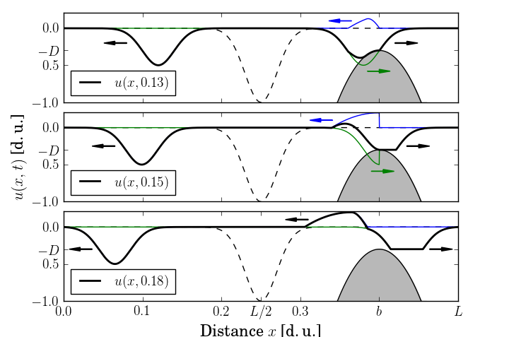
The video animation (.mp4 file, 1.7 MB) corresponding to Fig. 2 in the article and Fig. 1 presented here. The animation shows the evolution of the string displacement u(x,t) caused by the travelling waves r(x - ct) and l(x + ct). The time series result is shown for x = xr = L/2. Time t = tp shows the onset moment of the periodic vibration regime.
|
|
|
Figure 1. Reflection of travelling wave r(x - ct), shown with the thin green line, from the obstacle positioned at x = b shown with the grey formation. The refleted travelling wave l(x + ct) is shown with the thin blue line. Arrows indicate the directions of wave propagation. Bell-shaped initial condition is shown with the dashed line.
|
|
Effect of the obstacle radius
|
|
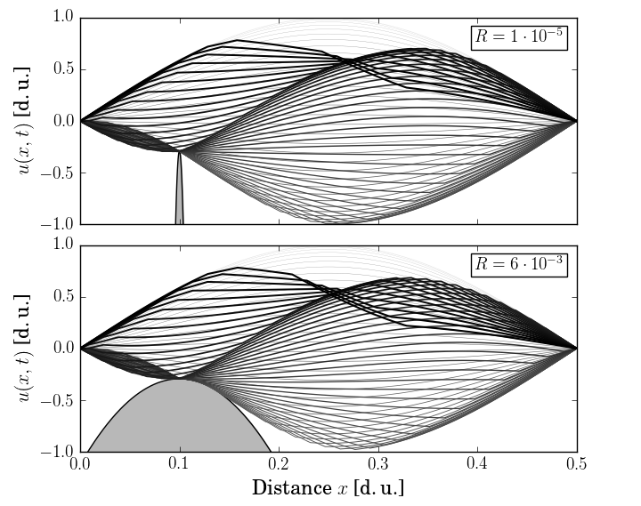
The video animation (.mp4 file, 8.7 MB), where obstacle radius R = 0.00001, and video animation (.mp4 file, 8.7 MB), where obstacle radius R = 0.006, corresponding to Fig. 3 and 4 in the article and Fig. 2 presented here. The time series result is shown for x = xr = 0.47 L. Time t = tp shows the onset moment of the periodic vibration regime. The result shown with the dotted line corresponds to the linear case, where the obstacle is absent.
|
|
|
Figure 2. Stroboscopic plot of the string displacement during the first period of vibration. Showing 68 time steps. The thickness of the lines is proportional to the direction of time flow. The obstacles with radius R = 0.00001 (top) and R = 0.006 (bottom) are positioned at b = L/5 and D = u(b,0)/2.
|
|
Effect of the obstacle proximity
|
|
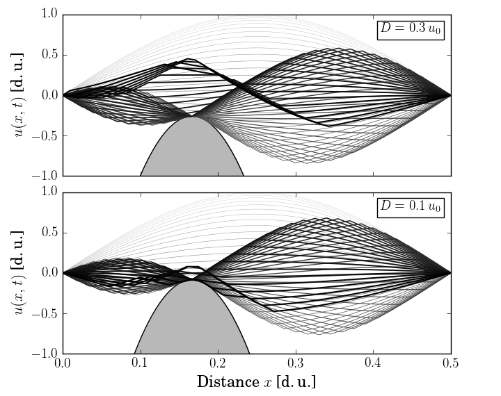
The video animation (.mp4 file, 8.6 MB), where obstacle proximity D = 0.3 u(b,0), and video animation (.mp4 file, 8.6 MB), where obstacle proximity D = 0.1 u(b,0), corresponding to Fig. 5 and 6 in the article and Fig. 3 presented here. The time series result is shown for x = xr = 0.47 L. Time t = tp shows the onset moment of the periodic vibration regime. The result shown with the dotted line corresponds to the linear case, where the obstacle is absent.
|
|
|
Figure 3. Stroboscopic plot of the string displacement during the first period of vibration. Showing 68 time steps. The thickness of the lines is proportional to the direction of time flow. The obstacle with radius R = 0.003 is positioned at b = L/3. The obstacle with proximity D = 0.3 u(b,0) (top) and D = 0.1 u(b,0) (bottom) are presented.
|
|
Effect of the obstacle position along the string
|
|
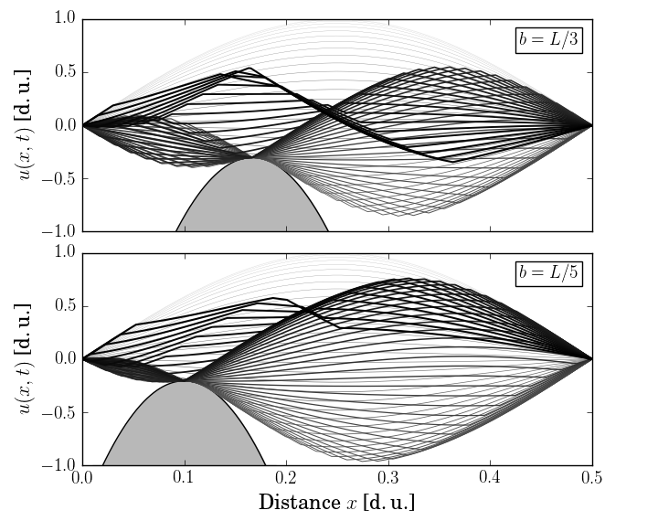
The video animation (.mp4 file, 8.6 MB), where obstacle position b = L/3, and video animation (.mp4 file, 8.6 MB), where obstacle position b = L/5, corresponding to Fig. 7 and 8 in the article and Fig. 4 presented here. The time series result is shown for x = xr = 0.47 L. Time t = tp shows the onset moment of the periodic vibration regime. The result shown with the dotted line corresponds to the linear case, where the obstacle is absent.
|
|
|
Figure 4. Stroboscopic plot of the string displacement during the first period of vibration. Showing 68 time steps. The thickness of the lines is proportional to the direction of time flow. The obstacle with radius R = 0.004 is positioned at b = L/3 (top) and b = L/5 (bottom), and in both cases D = 0.35 u(b,0).
|
|
Symmetric case (not presented in the article)
|
|
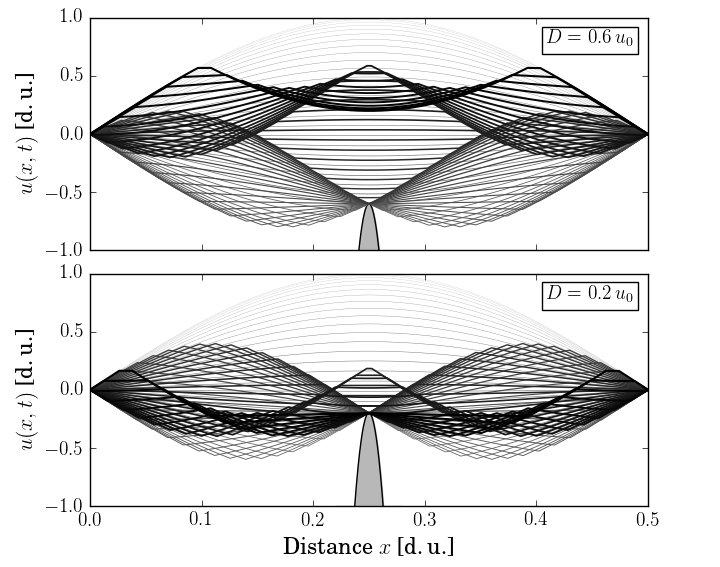
The video animation (.mp4 file, 8.7 MB), where obstacle proximity D = 0.6 u(b,0), and video animation (.mp4 file, 8.6 MB), where obstacle proximity D = 0.2 u(b,0), corresponding to Fig. 5 presented below. In both cases the obstacle is positioned at x = b = L/2. The time series result is shown for x = xr = 0.47 L. Time t = tp shows the onset moment of the periodic vibration regime. The result shown with the dotted line corresponds to the linear case, where the obstacle is absent.
|
|
|
Figure 5. Stroboscopic plot of the string displacement during the first period of vibration. Showing 72 steps. The thickness of the lines is proportional to the direction of time flow. The obstacle with radius R = 0.0001 is positioned at b = L/2. The obstacle with proximity D = 0.6 u(b,0) (top) and D = 0.2 u(b,0) (bottom) are presented.
|
|
Conclusions
|
In this paper the kinematics of ideal string vibration against an absolutely rigid obstacle was modeled using the approach based on the application of the d’Alembert formula as explained in Sec. 3. The presented numerical method is accurate and efficient lacking numerical dispersion caused by accumulative approximation errors. The effect of the obstacle proximity D on the string vibration and on the mean level of upper mode amplitudes was clearly evident and this was to confirm that the problem is nonlinear.
It was shown that the ideal lossless string interacting with the obstacle vibrates in two distinct vibration regimes. In the beginning of the kinematic interaction between the vibrating string and the obstacle the string motion is aperiodic with constantly evolving spectrum. After some time of aperiodic vibration the string vibration settles in the periodic regime where the string motion is repetitious in time. The duration of the aperiodic regime depends on the obstacle proximity D, position b, and geometry (curvature radius R). The comparison of the resulting spectra in the periodic regime with the linear case where the obstacle was missing showed that the general effect of the obstacle manifests in the widening of the spectrum caused by transfer of fundamental mode energy to upper modes. The analysis of the relatively short-lasting aperiodic regime showed that the obstacle position b may generate temporary fractional subharmonics related to the node point at x = b. In conclusion, the results presented in this paper can expand our understanding of timbre evolution of numerous stringed instruments, such as, the guitar, bray harp, tambura, veena, sitar, etc. The possible applications include, e.g., sound synthesis of these instruments.
|
|
This research was supported by the Estonian Ministry of Education and Research, Project IUT33-24, and by Doctoral Studies and Internationalisation Programme DoRa Plus Action 1.1 (Archimedes Foundation, Estonia) through the ERDF. The author is grateful to the anonymous reviewers of this paper—their suggestions improved the manuscript greatly.
|


|
Kinematics of ideal string vibration against a rigid obstacle (DAFx-17)
|